Approximating Translucency Revisited – With “Simplified” Spherical Gaussian Exponentiation

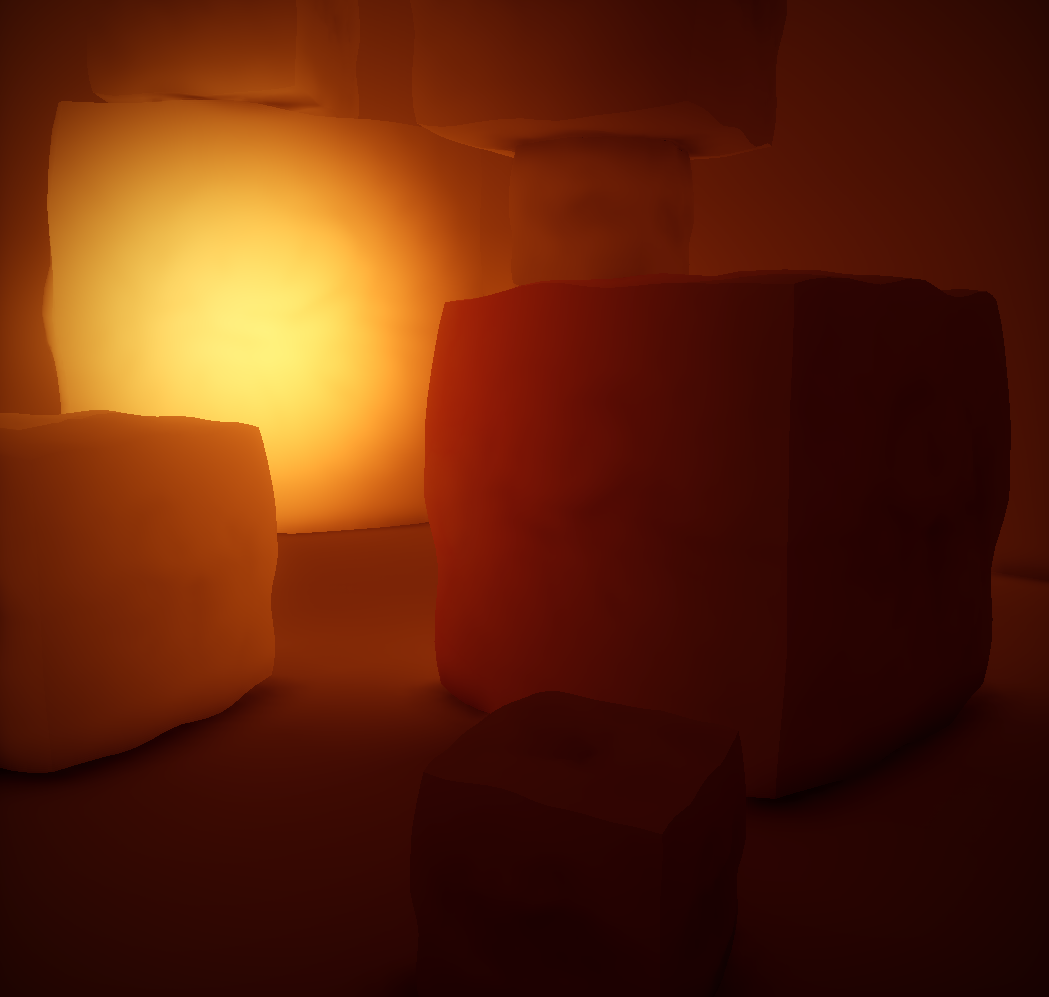
Lately, someone at work has pointed out the approximation of translucency Marc Bouchard and I developed back at EA [1], which ended up in DICE’s Frostbite engine [2] (aka The Battlefield 3 Engine). Wanting to know more, we started browsing the slides one by one and revisiting the technique. Looking at the HLSL, an optimization came to my mind, which I’ll end up discussing in this post. In case you missed the technique, here’s a few cool screenshots made by Marc, as well as tips & tricks regarding implementing the technique and generating the inverted ambient-occlusion/thickness map. See the references for additional links.

As mentioned in [2], the approximation of translucency is implemented as such:

// fLTDistortion = Translucency Distortion Scale Factor 
// fLTScale = Scale Factor 
// fLTThickness = Thickness (from a texture, per-vertex, or generated) 
// fLTPower = Power Factor
half3 vLTLight = vLight + vNormal * fLTDistortion;
half fLTDot = pow(saturate(dot(vEye, -vLTLight)), fLTPower) * fLTScale;
half3 fLT = fLightAttenuation * (fLTDot + fLTAmbient) * fLTThickness;
half3 cLT = cDiffuseAlbedo * cLightDiffuse * fLT;

In parallel, as mentioned in Christina Coffin’s talk on tiled-based deferred shading for PS3 [3], Matthew Jones (from Criterion Games) provided an optimization to computing a power function (or Exponentiation, i.e. for specular lighting) using a Spherical Gaussian approximation. This was also documented by Sébastien Lagarde [4][5]. By default, pow is roughly/generally implemented as such:

// Generalized Power Function
float pow(float x, float n)
{
    return exp(log(x) * n);
}

The Spherical Gaussian approximation replaces the log(x) and the exp(x) by an exp2(x). The specular power (n) is also scaled and biased by 1/ln(2):

// Spherical Gaussian Power Function float pow(float x, float n)
{
    n = n * 1.4427f + 1.4427f; // 1.4427f --> 1/ln(2)
    return exp2(x * n - n);
}

If possible, you should handle the scale and bias offline, or somewhere else. Additionally, if you have to compute the scale and bias at runtime, but don’t really care what actual number is passed as the exponent, a quick hack is to get rid of the scale and the bias all-together. While this is not something you necessarily want to do with physically-based BRDFs – where exponents are tweaked based on surface types – in the case you/artists are visually tweaking results (i.e. for ad hoc techniques, such as this approximation of translucency), this is totally fine. In our case, artists don’t care if the value is 8 or 12.9843 (8*1.4427+1.4427), they just want a specific visual response, and it saves ALU. Again, not to be used for all cases of pow(x, n), but you should try it with other techniques. You’d be surprised how much people won’t see a difference. 🙂

In the end, after injecting the “Simplified” Spherical Gaussian approximation in our translucency technique, we get:

// fLTDistortion = Translucency Distortion Scale Factor 
// fLTScale = Scale Factor 
// fLTThickness = Thickness (from a texture, per-vertex, or generated) 
// fLTPower = Power Factor
half3 vLTLight = vLight + vNormal * fLTDistortion;
half fLTDot = exp2(saturate(dot(vEye, -vLTLight)) * fLTPower - fLTPower) * fLTScale;
half3 fLT = fLightAttenuation * (fLTDot + fLTAmbient) * fLTThickness;
half3 cLT = cDiffuseAlbedo * cLightDiffuse * fLT;

References

[1] BARRÉ-BRISEBOIS, Colin and BOUCHARD, Marc. “Real-Time Approximation of Light Transport in Translucent Homogenous Media”, GPU Pro 2, Wolfgang Engel, Ed. Charles River Media, 2011.

[2] BARRÉ-BRISEBOIS, Colin and BOUCHARD, Marc. “Approximating Translucency for a Fast, Cheap and Convincing Subsurface Scattering Look”, GDC 2011, available online.

[3] COFFIN, Christina. “SPU-based Deferred Shading for Battlefield 3 on Playstation 3”, GDC 2011, available online.

[4] LAGARDE, Sébastien. “Adopting a physically based shading model”, Personal Blog, available online.

[5] LAGARDE, Sébastien. “Spherical gaussien approximation for Blinn-Phong, Phong and Fresnel”, available online.