As of today, HLSL doesn’t officially support constructors for user-created classes. In the meantime, with the current tools at our disposal, maybe there is a way to work around this limitation and emulate constructor functionality ourselves?
It turns out we can!
This post describes how to implement constructor-like* functionality in HLSL. The following implementation relies on Microsoft’s DirectX Shader Compiler (DXC) and works for default constructors and constructors with a variable number of arguments.
Note: constructor-like is essential here. Not all functionality is supported, but enough to make it meaningful and worth your while.
Constructor Support in HLSL
Currently, constructors are only available for native HLSL types such as vector and matrix types:
bool2    u = bool2(true, false);
float3   v = float3(1, 2, 3);
float4x4 m = float3x3(1,0,0,0,0,1,0,0,0,0,1,0,0,0,0,1);
For example, the following is not supported (yet):
class MyClass
{
public:
    // Default Constructor
    MyClass()
    {
        x = 0;
        b = false;
        i = 0;
    }

    // Constructor with a single parameter
    MyClass(const float inX) : MyClass()
    {
        x = inX;
    }

    // Constructor with multiple parameters
    MyClass(const float inX, const bool inB, const int inI)
    {
        x = inX;
        b = inB;
        i = inI;
    }

private:
    // Member variables
    float x;
    bool  b;
    int   i;
};

MyClass a = MyClass();              // Default Constructor
MyClass b = MyClass(3.0f);          // Constructor with a single parameter
MyClass c = MyClass(3.0f, true, 7); // Constructor with multiple parameters
At compilation, several errors will appear due to the lack of functionality.
So, typically, workarounds come in different shapes or forms:
// Initializes the whole class to 0
MyClass a = (MyClass)0;

// Initializes an instance of the class via another function,
// with single parameter
MyClass CreateMyClass(const float x)
{
    MyClass a;
    a.x = x;
    return a;
}
MyClass b = CreateMyClass(3.0f);

// Initializes an instance of the class via another function,
// with multiple parameters
MyClass CreateMyClass(float inX, bool inB, int inI)
{
    MyClass a;
    a.x = inX;
    a.b = inB;
    a.i = inI;
    return a;
}
MyClass b = CreateMyClass(3.0f, true, 7);
While this might be fine for a simple case, it really adds up in bigger codebases. Also, wouldn’t it be great if these functions could live together with the class they initialize like a typical constructor does? HLSL supports public classes implemented via structs, where member functions are possible. For sure we can do better.
Implementing HLSL Constructors
It turns out that constructors can be emulated in DXC using variadic macros, from LLVM, and with a bit of elbow grease. Let’s adjust our previous example:
#define MyClass(...) static MyClass ctor(__VA_ARGS__)
class MyClass
{
    // Default Constructor
    MyClass()
    {
        return (MyClass)0;
    }

    // Constructor with a single parameter
    MyClass(const float x)
    {
        MyClass a = MyClass();
        a.x = x;
        return a;
    }

    // Constructor with multiple parameters
    MyClass(const float x, const bool b, const int i)
    {
        MyClass a;
        a.x = x;
        a.b = b;
        a.i = i;
        return a;
    }

    // Member variables
    float x;
    bool  b;
    int   i;
};
#define MyClass(...) MyClass::ctor(__VA_ARGS__)
Note: public and private are reserved keywords in HLSL. Currently, classes are structs.
How Does it Work?
First, at Line 1, the macro handles the typical signature one would expect from a constructor. The variadic ... and __VA_ARGS__ enables the definition of constructors-like member functions with a variable number of parameters. At compilation, this replaces all following calls of MyClass(…) with static MyClass ctor(...).
Then, line #33 redefines the MyClass(...) static member function(s), so they can be used later in the code. We are now able to call MyClass(...) directly, which creates and initializes an instance of that class:
MyClass a = MyClass();              // Default Constructor
MyClass b = MyClass(3.0f);          // Constructor with a single parameter
MyClass c = MyClass(3.0f, true, 7); // Constructor with multiple parameters
Success!
Further Simplification
If one wants to eliminate the generic zero-ing default constructor, further simplification is possible with this macro:
#define DEFAULT_CONSTRUCTOR(Type) static Type ctor() { return (Type)0; }
This optional macro further helps remove code deduplication, especially as one implements many classes throughout a big HLSL codebase.
#define MyClass(...) static MyClass ctor(__VA_ARGS__)
class MyClass
{
    // Default Constructor
    DEFAULT_CONSTRUCTOR(MyClass);

    ...
Wrapping-Up & Additional Thoughts
This post demonstrates an implementation of constructor-like functionality in HLSL that works with out-of-the-box DXC.
Woohoo!
Now, as you probably noticed it lacks some functionality to fully cover what constructors enable. But it’s close!
In the event where you have your own HLSL parser, you might be able to work around this whole problem altogether. You could, for example, as a precompilation step, parse your entire codebase and create, build, and call constructors with unique signatures to prevent name collisions. In my case, I wanted to build something that would work out of the box with vanilla DXC. This is what the previous examples solve.
Also, it would be nice if recursive macros were supported. One could use recursive macros to generalize the two #define above and possibly eliminate the various return calls. Unfortunately, recursive macros are not available.
Either way, I’ve been experimenting with this approach for a few months now, and I have found it quite helpful. I find it cleans up usage of user-created classes and brings us one step closer. I hope you find it helpful too!
Until we get native support for constructors in HLSL, please post in the comments if you manage to improve or simplify this approach further or stumble on a more straightforward way. Thanks!
PS: Thanks to Jon Greenberg for reviewing this small blog post.
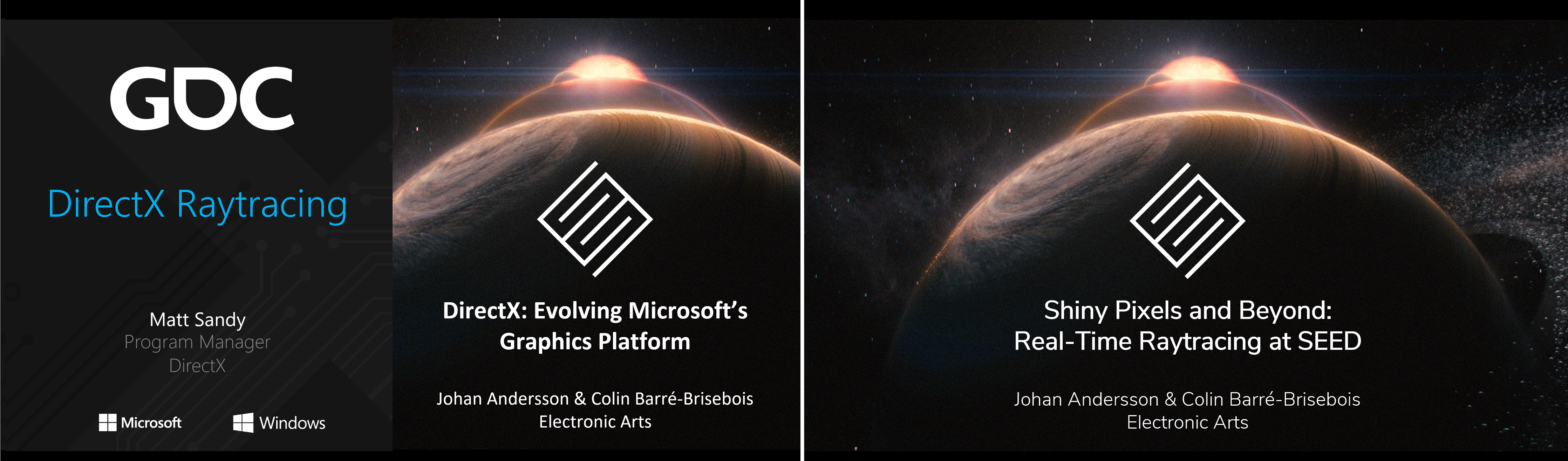 DirectX Raytracing Announcement (Microsoft) and Shiny Pixels and Beyond: Real-Time Raytracing at SEED (NVIDIA)
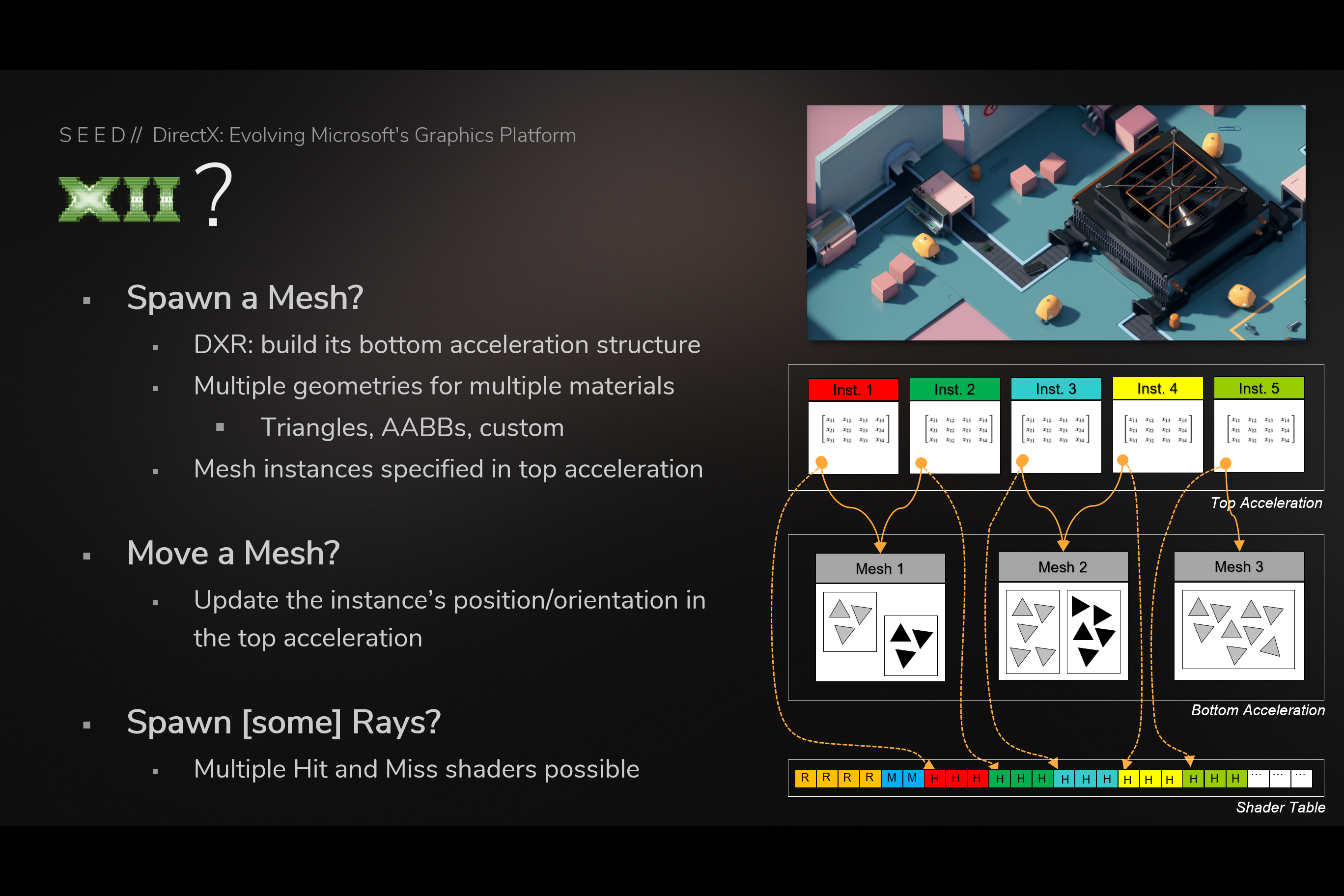 Using Bottom/top acceleration structures and shader table (from GDC slides)
 Ray Generation Shadow – HLSL Pseudo Code – Does Not Compile (from GDC slides)
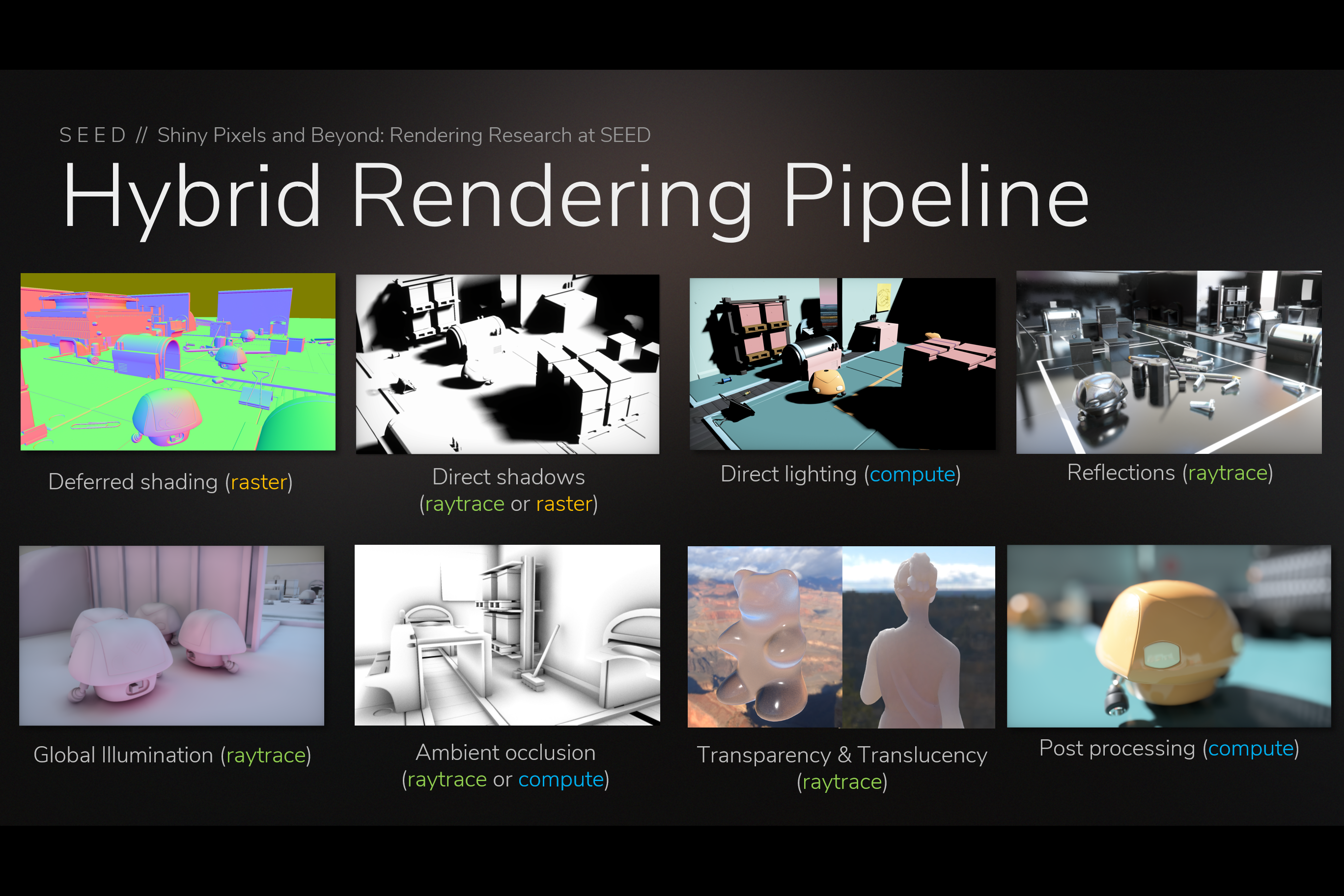 PICA PICA’s Hybrid Rendering Pipeline (from GDC slides)
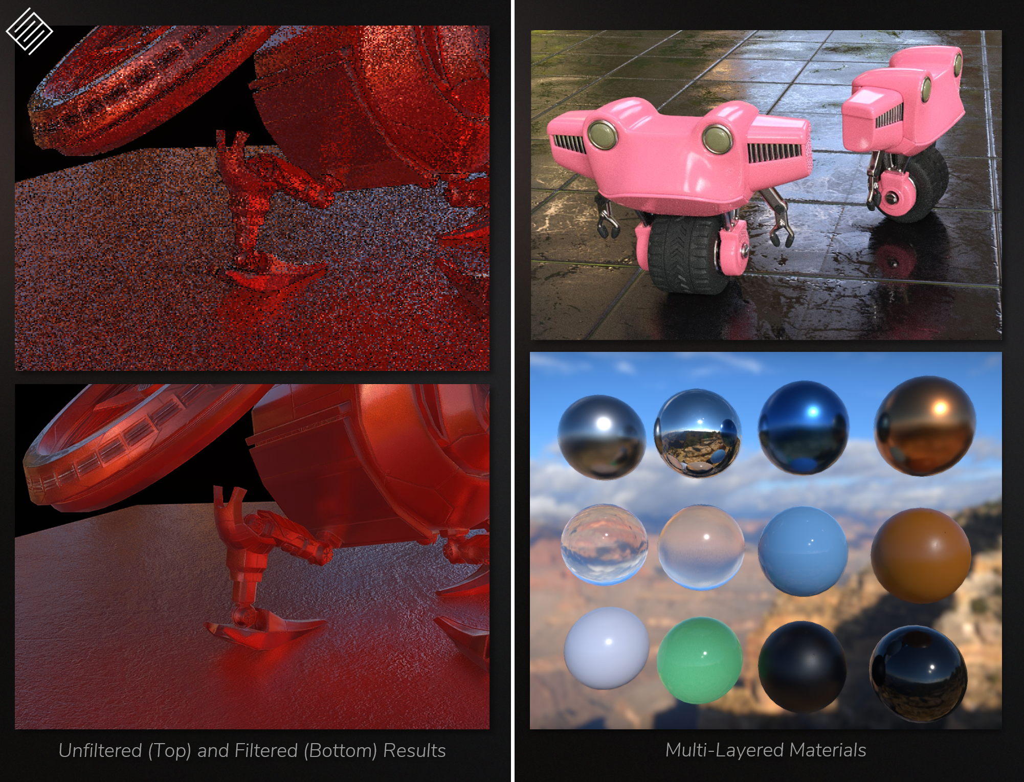 Raytraced Reflections (left) and Multi-Layer Materials (right) (from GDC slides)
 Glass and Translucency (from GDC slides)
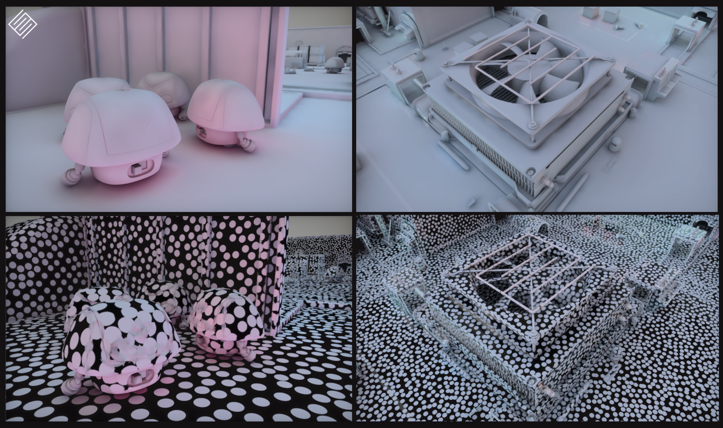 Surfel-based Global Illumination (from GDC slides)
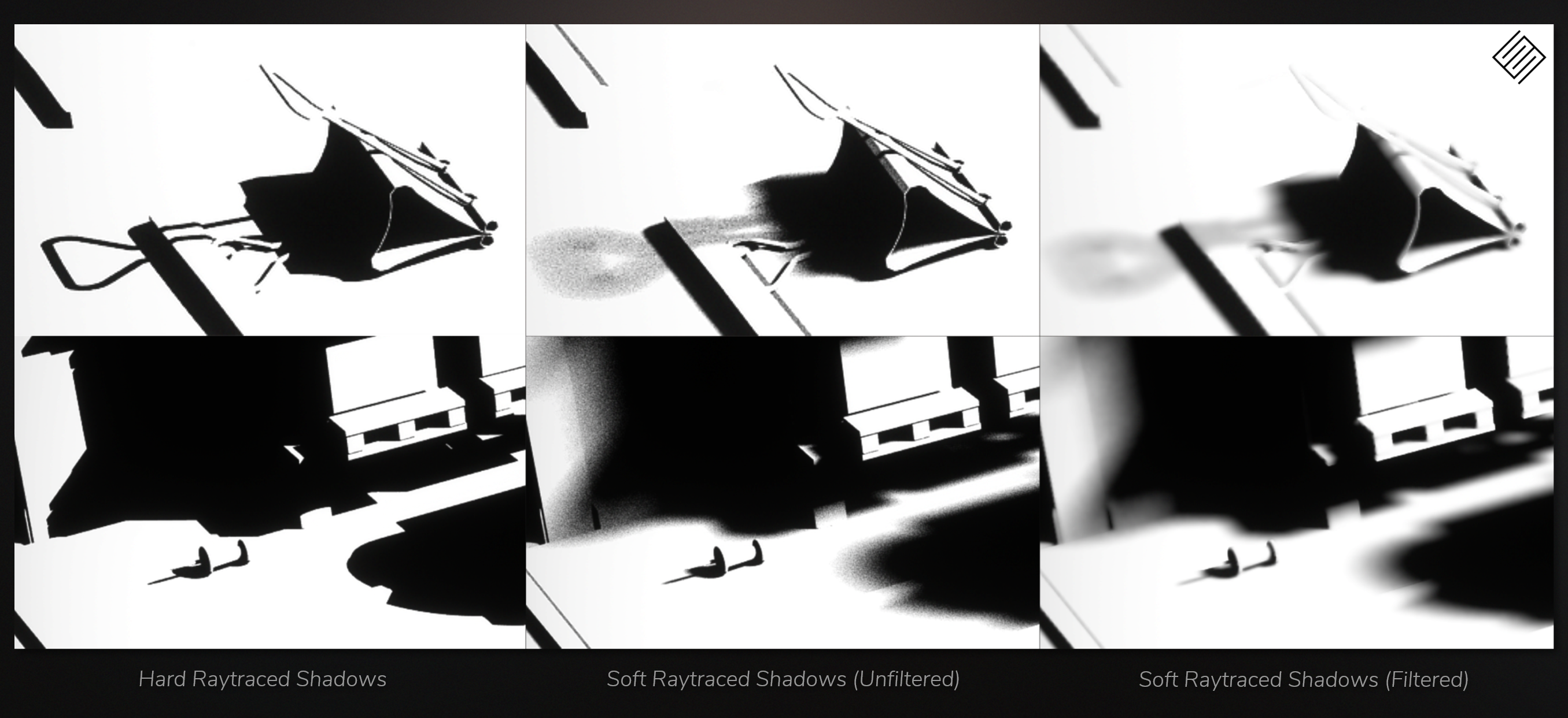 Surfel-based Global Illumination (from GDC slides)
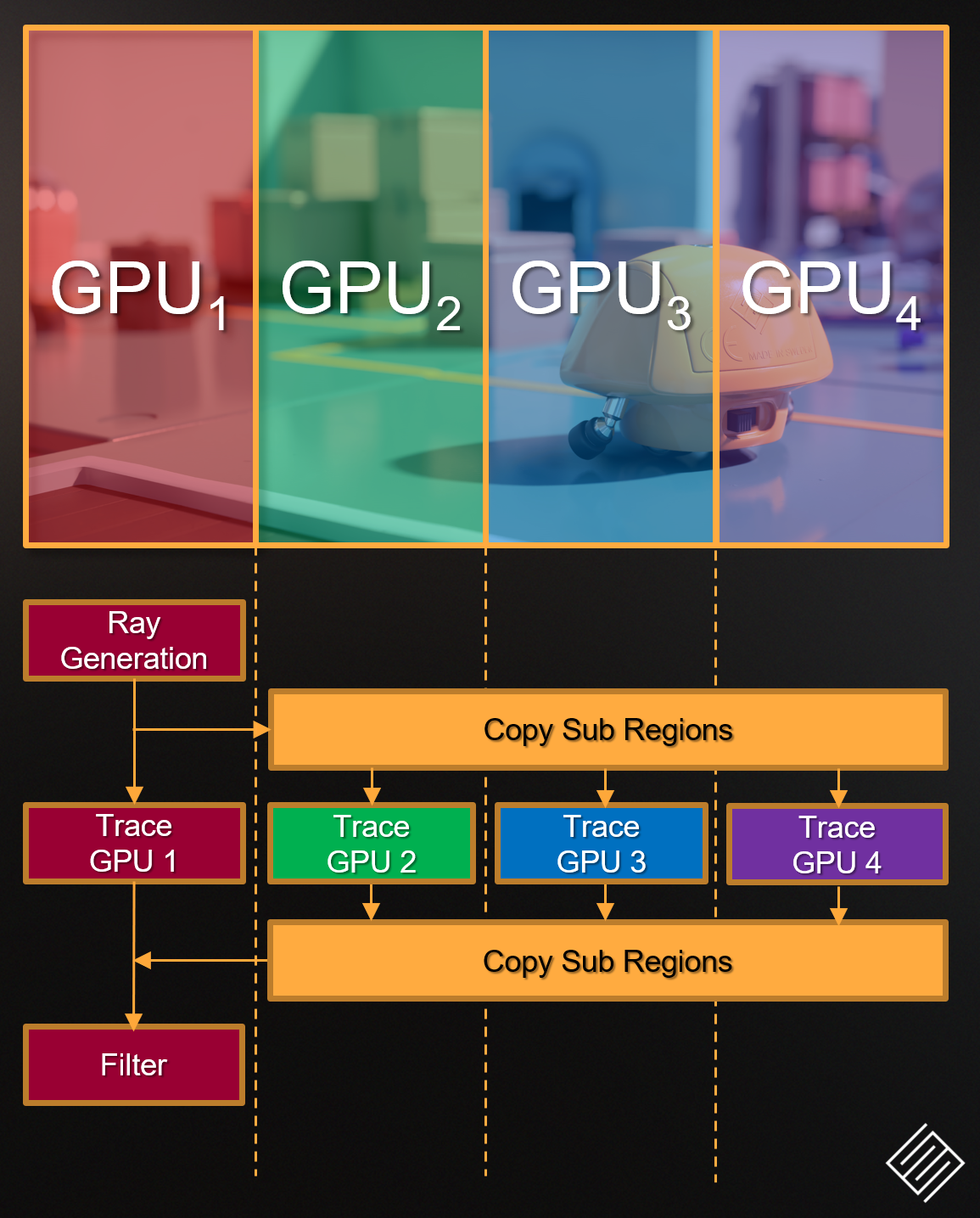 mGPU in PICA pica (from GDC slides)
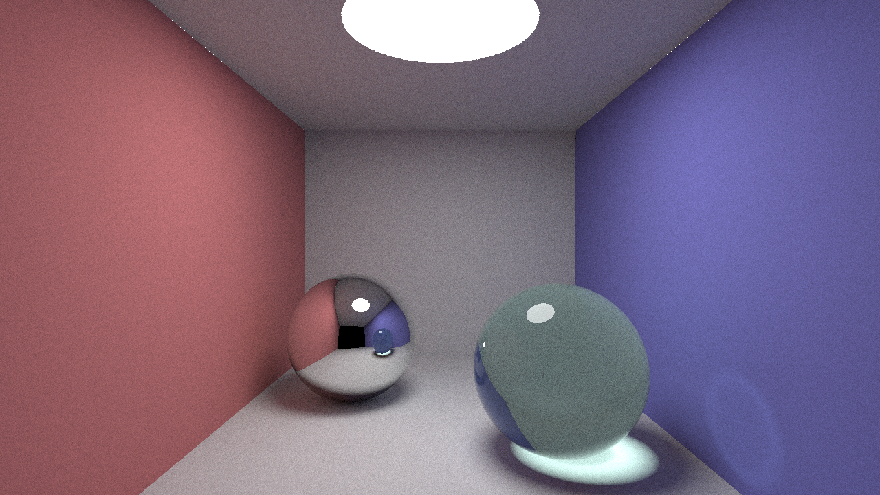


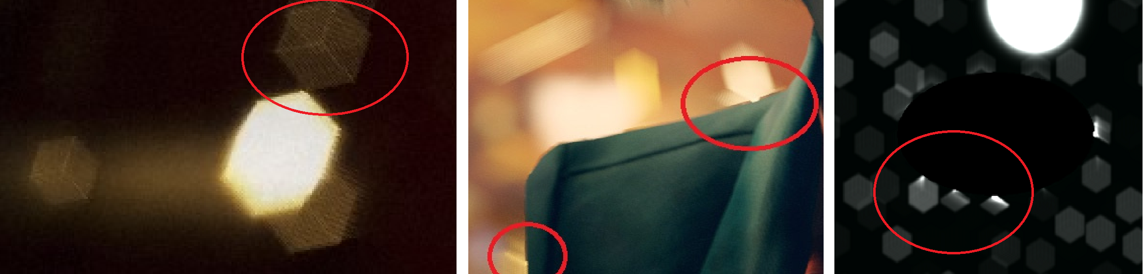
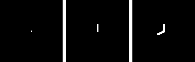
 Y-shaped Artifact
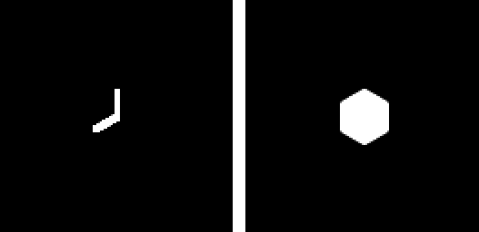
 Rhombi Overlap (Left) vs Proper Alignment (Right)
 Rotated Hexagonal Bokeh Depth-of-Field in Ghost Recon Wildlands


 Tom Clancy’s The Division – Ubisoft